How to Make a Bar Graph in Excel

Excel's chart features can turn your spreadsheet data into compelling visual communications—if you know what to do. This guide will walk you through the basics of setting up trends, percentages, relationships, averages, and much more. We'll keep adding information over time, so bookmark this page to learn more.

Chart Designs

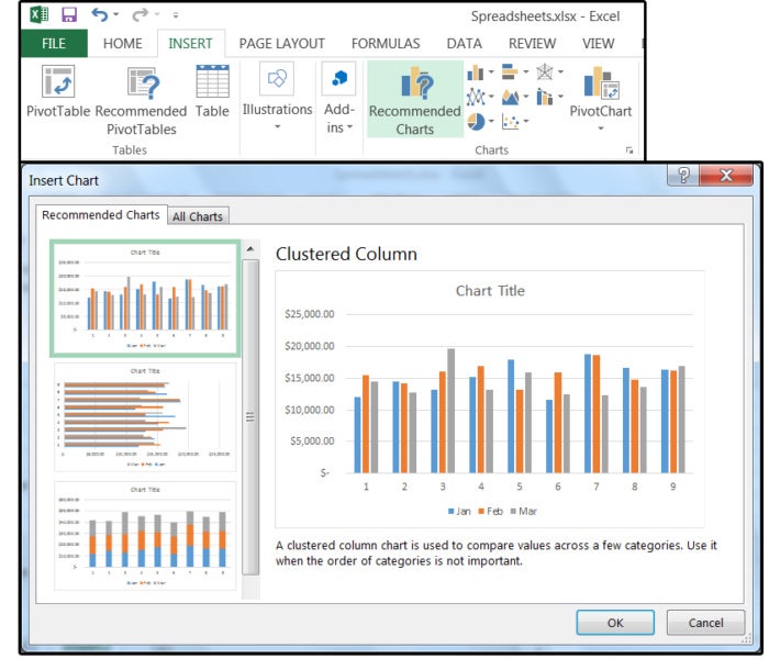
Excel has 16 chart designs with several models in each design, plus a dozen or so styles, colors, and layouts for each model in each design. According to Microsoft, specific types of data are paired with the chart design that showcases that data best. When you select Recommended Charts from the Insert tab, Excel displays a visual list of the charts that would most successfully represent your current dataset.

For example, Column charts illustrate how data changes over time, but they're also the best design to show comparisons among items. Bar charts are, essentially, just horizontal Column charts and are generally used when the axis labels are exceptionally long. Pie charts are used to show percentages of the whole, and Line charts excel with data trends.

The remaining chart designs include Area, Stock, Surface, Combo, Pareto, Histogram, and Sunburst. For best results, avoid the following designs altogether: Radar, Bubble, XY/Scatter, Treemap, Waterfall, and Box & Whisker. These six chart designs are so difficult to read, they fail to explain the data to most viewers.

01 recommended charts — Recommended Chart designs include the classic Column variety.

Chart Structure

Before we tackle individual chart designs and models, it's important to understand how charts are constructed. Composed from your databases, which contain fields (columns) and records (rows), charts are comprised of categories, which are generally aligned along the horizontal axis, and values (or data series), which line up along the vertical axis. Let's build a quick chart to show how all the pieces function.

1. Highlight the columns and rows in your Excel database that you want to chart. In our example (below), we highlighted columns B through D and rows 2 through 11 (the names of the months and the sales dollars of each month (that is, B2:D11).

2. Click Insert > Recommended Charts and select a design from the Chart List. For simplicity, choose the first design on the list (the Clustered Column), then click OK.

3. Excel drops the chart into the middle of the screen. Click the chart to activate it.

4. Position your cursor on one of the double-lined borders and, when the cursor turns into a cross with arrow tips, hold down the left mouse button and drag the chart to wherever you like.

5. Notice the three icons on the right side of the chart: Elements, Chart Styles, and Series/Categories.

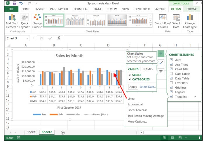
6. With the chart is selected, click the green plus sign and the Chart Elements menu pops up.

7. The Elements of the chart include the Axis and the Axis Titles (primary horizontal & vertical), the Chart Title, the Data Labels, Gridlines, the Legend, and a Trend line (with several options under each element).

8. Check or uncheck the boxes to activate or deactivate the individual Elements.

9. Scroll down the list and notice the small gray arrows that appear beside each element. Click those arrows to open submenus with additional options for each element.

10. When you check the boxes for titles (axis and chart), you're prompted to type your custom information for those titles. Enter those titles now.

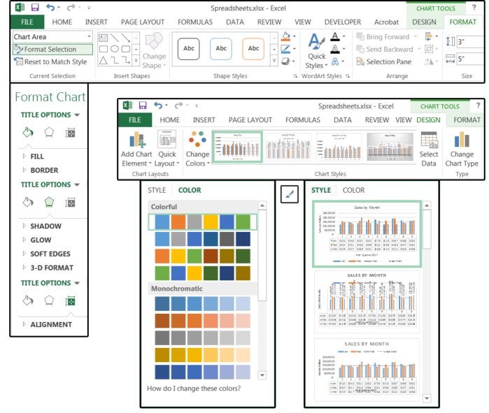
11. Click the paintbrush (Chart Styles) button, and the Style and Color menu pops up. From this menu, you can change the design styles and colors. You can also make these changes through the Chart Tools menus.

12. When the chart is selected, two new tabs appear on the Ribbon menu: Chart Tools Design and Chart Tools Format. The Design menu also shows the Styles and Colors options, plus Chart Layout, the option to add Chart Elements, and several other features.

13. The Chart Tools Format tab is for the chart text, such as the titles and data labels. From this menu. you change the font typeface, color, size, style, and special effects. Or you can click the Format Selection icon (far left) and open the menu, which includes the borders, fill, alignment, and text effects such as Shadow, Glow, Edges, and 3D Format.

03 chart tools design format — Chart Tools Design and Format

14. You can also access all of these features through the shortcut keys. Use the Alt key to access the shortcut menu, which displays shortcut letters inside black boxes.

Note the proper way to use shortcut keys. For example, to access the charts, type Alt-N-R. The hyphens designate this command as a consecutive combo keystroke. In other words, press the Alt key and release; then press the N and release; then press the R and release.

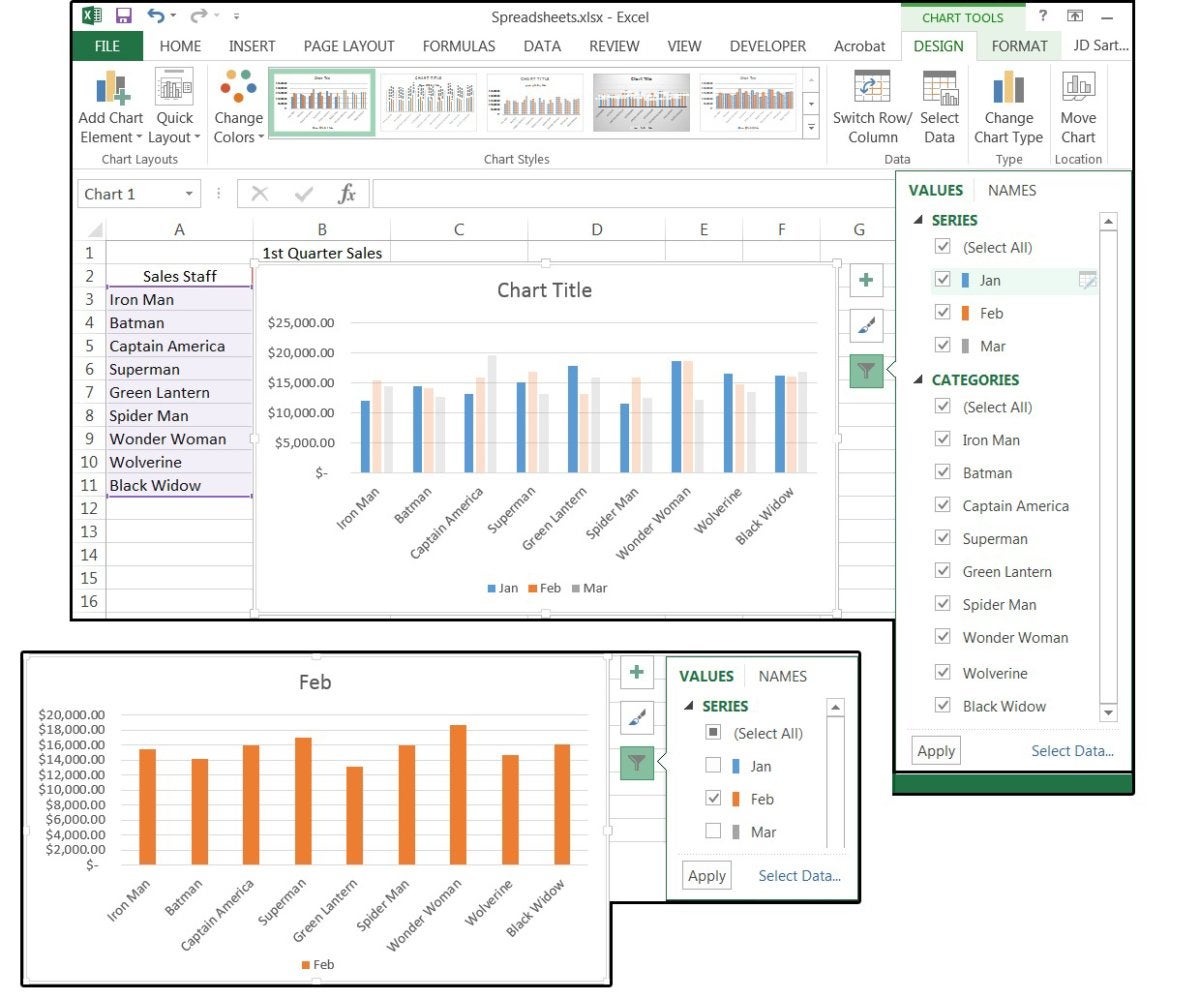
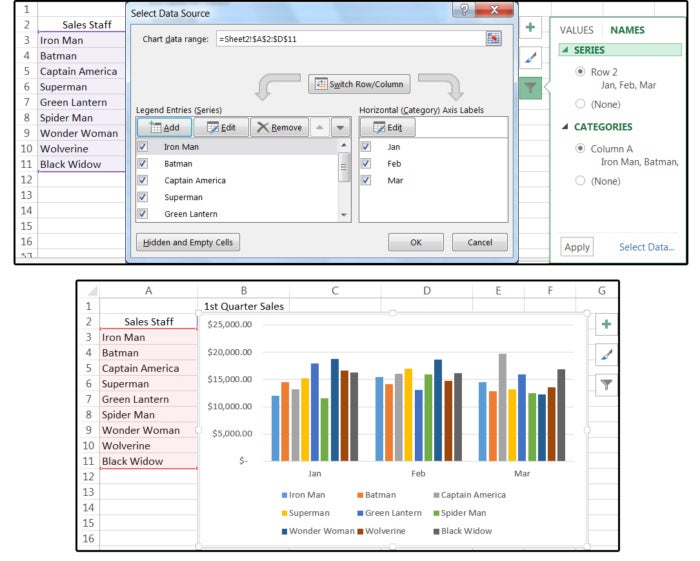
15. With the chart still selected, click the funnel (Chart Filters) button, and the Values and Names menu pops up. Use the Values menu to view and/or modify the Series (Jan, Feb, Mar) or Categories (from Iron Man through Black Widow). If you scroll down and hover over any single Series (such as Jan) or Category, notice that the other months/categories fade. If you uncheck any of the Series or Categories, only the checked items are charted. Click Apply when finished.

04 use the chart filters button to filter series or categories — Use the Chart Filters button to filter Series and Categories

16. Use the Names tab to change the names of the Series or Categories, or select None to get generic names such as Series 1, 2, 3 or Category 1, 2, 3, etc..

17. Click the Select Data link (bottom right corner) of the Chart Filters menu to alter (add, edit, remove) fields or records in your database. You can also switch or exchange) the column data with the row data. For example, you can chart each employee's sales by month. Or, you can switch the columns and rows and chart each month's sales by employee (such as Jan sales for each employee).

This is a handy feature to use if, suddenly, your boss says, "Yeah, but how do the employees' sales compare to one another each month?" Instead of reworking your spreadsheet or redesigning your chart, you can click one button and completely change the way the charted data displays.

05 click the select data link to reverse the columns rows — Click the Select Data link to reverse the columns and rows

For this initial Charts piece, we'll cover the most popular and user friendly chart designs, including all the models within each of those designs.

Column & Bar charts

Column and Bar charts are identical, except Columns are vertical and Bars are horizontal. They're available in six styles: Clustered, Stacked, 100% Clustered, 3D Clustered, 3D Stacked, and 3D 100% Stacked. Column also has one more: plain 3D style.

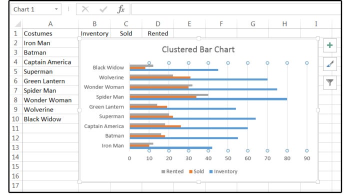
1. The Clustered column/bar and 3D clustered column/bar charts are in 2D and 3D formats, respectively. Use these charts for scaled data (called the Likert Scale) such as those used in polls. This chart is also useful for ranges of numbers or data and/or items that are not in any explicit order.

2. The Stacked column/bar and 3D stacked column/bar also show values in 2D and 3D formats. This chart is best for multiple data series with accentuated totals, or use it to separate and compare parts of a whole (like a pie chart). It's also effective for showing a grouped structure with a hierarchy that's one level deep.

06 clustered bar chart compares values across few categories — Clustered Bar chart compares values across minimal categories.

3. Stacked column/bar and 3D stacked column/bar charts are particularly useful for comparing the percentages of each value in a total. This means that the cumulative pieces of each stacked element always equals 100 percent. Also, notice how percentage values change over a period of time.

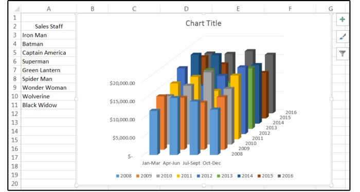
4. 3D column

The real plus for 3D charts—other than the obvious fact that they look so much cooler than 2D charts—is the added benefit of three axes (horizontal, vertical, and depth), which you can alter to fit your data. Use this chart to compare data across both categories and the data series.

07 the 3d column chart has three axeshorizontal vertical depth — The 3D Column chart has three axes—horizontal, vertical, and depth.

Pie Charts

The Pie chart is constructed from a single row (or column) of data that represents a part of the whole (pie); or a single column of numbers that, when added together, equal 100 percent. Or, to be more specific, the pie shows the size of items in one numeric series that's proportional to the sum of all the items.

Note: Pies can only chart one column (or row) of positive numbers. Negative values cannot be charted, and zero values should be minimal (one or two maximum). Last, the pie chart is limited to seven categories—that is, seven numbers that equal the whole.

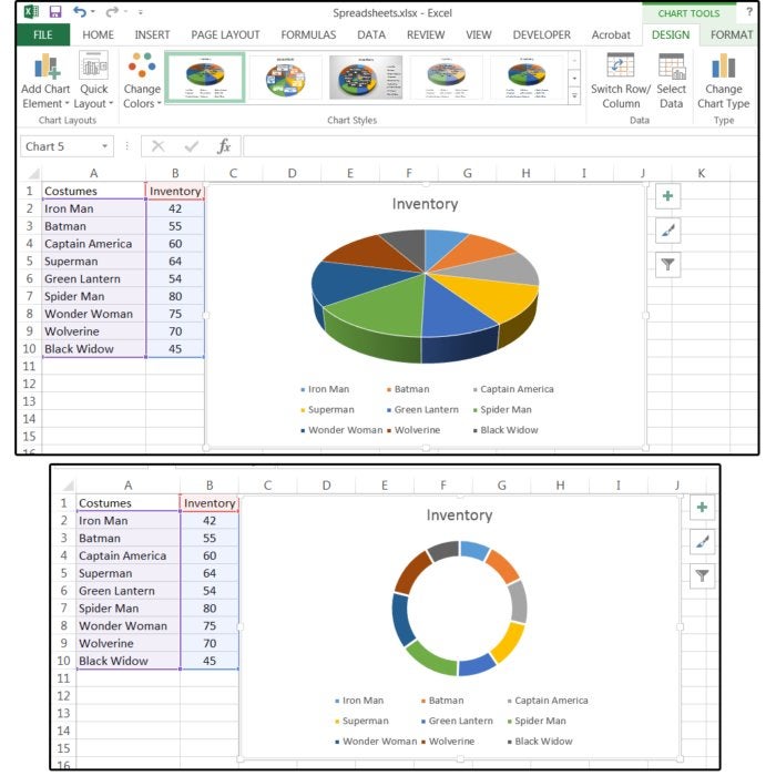
1. The Pie and 3D Pie charts are, obviously, in 2D or 3D format, and slices can be extracted for emphasis.

2. The Pie of Pie and Bar of Pie displays charts with smaller sections—of another pie or stacked bar chart—extracted from the whole, again, for emphasis.

3. The Doughnut charts also combine parts of a whole, but these charts can plot more than one column ordata series. The data is shown in rings, which each represent a data series; and each series totals 100 percent.

08 3d pie and donut charts — 3D Pie and Donut Charts

Line Charts

Line charts are pretty basic. The category info is dispersed (uniformly) along the horizontal axis, and the values are stacked evenly along the vertical axis. Because these charts can illustrate continuous data, over time, on an equally scaled axis, the Line chart is perfect for showing trends that occur in equivalent intervals such as time (morning, noon, midnight, etc.), dates (months, quarters, years, etc.), cycles (of the moon, planets, stars, etc.), seasons (spring, summer, autumn, winter), and so forth.

Use line charts when there are too many data points to plot in the other chart designs (such as column, bar, pie, etc.). If the categories need to be in a specific order, use a line chart instead of a clustered column or clustered bar; however, the clustered combo chart might work.

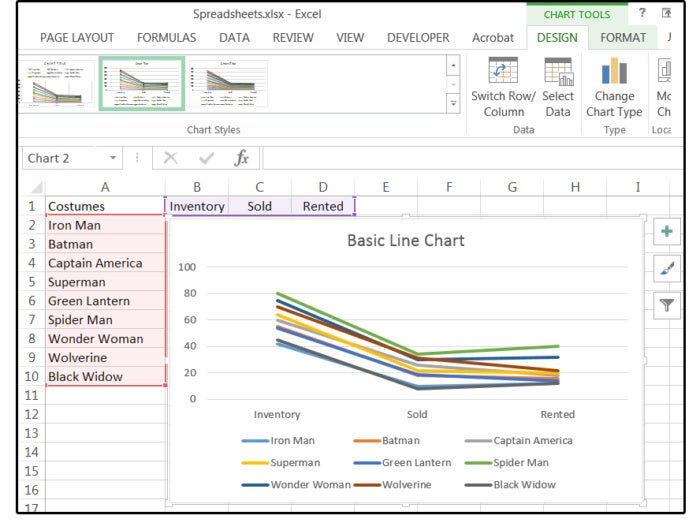
1. The Line and Line with markers charts show trends over time, evenly spaced categories, or data that must be presented in a specific order. For lots of categories or approximate values, omit the markers.

09 basic line chart without markers — Basic Line chart without markers

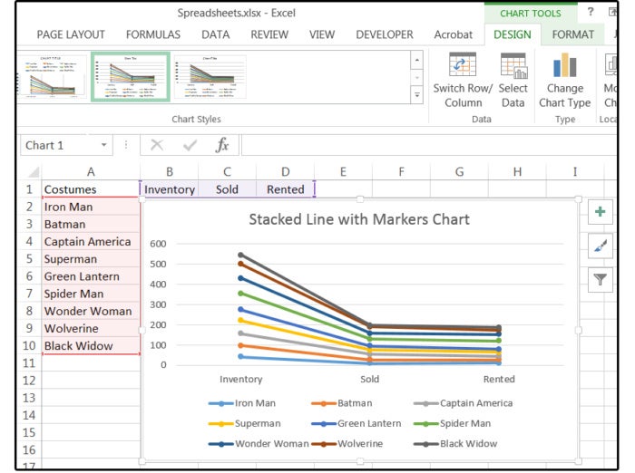
2. Stacked Line and Stacked Line with markers also show timely trends and evenly spaced categories.

3. 100% Stacked Line and 100% Stacked Line with markers show percentage trends over time or equally spaced categories. Again, for lots of categories or approximate values, omit the markers.

4. 3D Line charts display each row/column of data as a 3D ribbon. Like the other 3D charts, the 3D Line chart has three axes (horizontal, vertical, and depth) that can be altered.

10 stacked line chart with markers — Stacked Line Chart with markers

How to Make a Bar Graph in Excel

Source: https://www.pcworld.com/article/3225466/excel-charts.html

Savige Thoulluse